A (naive) application of linear mixed models to genetics
The following shows an application of class LMM from the Ruby gem mixed_models to SNP data (single-nucleotide polymorphism) with known pedigree structures. The family information is prior knowledge that we can model in the random effects of a linear mixed effects model.
Data
I have simulated realistic SNP data with the simulation software SeqSIMLA, using the software cosi to generate a reference sequence, as advised in the SeqSIMLA tutorial.
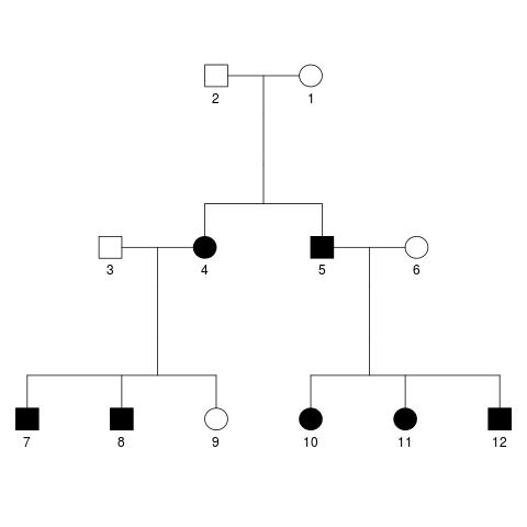
The response variable is a quantitative trait with mean 10 and variance 1. In total there are 130 SNPs in the data set, and SNPs 1, 3, 5 and 11 are selected to be causal, explaining 10%, 20%, 20% and 10% of the variance in the quantitative trait. Additionally, 35% of the variance is explained by shared environmental effects, and the remaining 5% by individual environmental effects. The correlation coefficient between spouses for the shared environmental effects is set to 0.8, and the respective correlation coefficients between parent and offspring as well as siblings is set to be 0.5. The data is available for ten families of twelve individuals each (i.e. 1200 subjects total). All families have identical pedigrees, which look like this:
The exact parameters provided to the SeqSIMLA software can be found in a text file in the repository. Additionally, I have preprocessed the SeqSIMLA output slightly and extracted the kinship matrix, both using a short R script.
The model
We model the quantitative trait \(y\) (a vector of length 1200) as,
\[y = X\beta + b + \epsilon,\]where \(X\) is a \(1200\times 130\) matrix containing the genotypes, \(\epsilon\) is a vector of i.i.d. random residuals with variances equal to \(\sigma\subscript{e}^2\), \(\beta\) is a vector of unknown fixed effects coefficients, and \(b\) is a vector of random effects.
If we denote the kinship matrix by \(K\), then we can express the probability distribution of \(b\) as
\[b\sim N(0, \sigma\subscript{b}^2 2K),\]where we multiply \(K\) by \(2\) because the diagonal of \(K\) is constant \(0.5\), and where \(\sigma\subscript{b}^2\) is a scaling factor.
The goal is to estimate the unknown parameters \(\beta\), \(\sigma\subscript{e}^2\) and \(\sigma\subscript{b}^2\), and to determine which of the fixed effects coefficients are significantly different from 0 (i.e. which SNPs are possibly causing the variability in the phenotype).
Fit the model in Ruby
First, we need to load the generated design matrix \(X\), the response vector \(y\), and the kinship matrix \(K\).
def read_csv_into_array(filename)
  f = File.new(filename)
  lines_array = Array.new
  f.each_line { |line| lines_array.push(line) }
  f.close
  lines_array.each_index do |i|
    lines_array[i] = lines_array[i].split(",")
    lines_array[i].each_index { |j| lines_array[i][j] = lines_array[i][j].to_f }
  end
  return lines_array
end

# fixed effects design matrix
x_array = read_csv_into_array("./data/design_matrix.csv")
n = x_array.length
m = x_array[0].length
x_array.unshift(Array.new(n) {1.0}) # intercept
x = NMatrix.new([n,m+1], x_array.flatten, dtype: :float64)

# response vector
y_array = read_csv_into_array("./data/phenotype.csv")
y = NMatrix.new([n,1], y_array.flatten, dtype: :float64)

# kinship matrix, which determines the random effects covariance matrix
kinship_array = read_csv_into_array("./data/kinship_matrix.csv")
kinship_mat = NMatrix.new([n,n], kinship_array.flatten, dtype: :float64)
Now, we can try to fit the model.
Instead of using the user-friendly method LMM#from_formula to fit the model, we will fit the model with raw model matrices directly using LMM#initialize. While LMM#from_formula mimics the behaviour of the function lmer from the popular R package lme4 (see my previous blog posts), LMM#initialize gives more flexibility to the user and allows for less conventional fits, which (to my knowledge) are not directly covered by lme4. This flexibility comes in form of an interface, where the user can supply the parametrization for the triangular Cholesky factor of the covariance matrix of the random effects in form of a Proc object or a block (which probably would not be as nice syntactically in most other languages as it is in Ruby).
In this case, the Cholesky factor of the covariance matrix is \(\sqrt{2} \sigma\subscript{b} \Lambda\), where \(\Lambda\) is the Cholesky factor of the kinship matrix \(K\). For convenience, we use the transformation \(\theta = \sqrt{2} \sigma\subscript{b}\).
Before we call LMM.new, we also need to define the random effects model matrix \(Z\) (which is the identity matrix in this case), find the Cholesky factor \(\Lambda\) of the kinship matrix \(K\), and specify the column names for the SNP matrix \(X\). These steps and the model fit are performed by the following Ruby code.
require 'mixed_models'

z = NMatrix.identity([n,n], dtype: :float64)

# upper triangulat Cholesky factor
kinship_mat_cholesky_factor = kinship_mat.factorize_cholesky[0]

# fixed effects names
x_names = [:Intercept]
1.upto(m) { |i| x_names.push("SNP#{i}".to_sym) }

# Fit the model
model_fit = LMM.new(x: x, y: y, zt: z,
                    x_col_names: x_names,
                    start_point: [2.0],
                    lower_bound: [0.0]) { |th| kinship_mat_cholesky_factor * th[0] }
It takes a couple of minutes to run.
Results
We can start by looking at some parameters describing the model fit:
puts "Optimal theta: \t#{model_fit.theta}"
puts "REML criterion: \t#{model_fit.deviance}"
yields
Optimal theta: 	[2.508012294769287]
REML criterion: 	3919.756682815396
(I know, not very meaningful to look at… At least, we see that the optimization method converged.)
Now, we might be interested to see which of the SNPs explain the variation in the quantitative trait best. To this end, we print those SNPs to the screen, which have a Wald p-value less than 0.05 (I have written before about Wald Z tests not being adequate, also see update below).
p_vals = model_fit.fix_ef_p
p_signif = Array.new
p_vals.each_key { |k| p_signif.push(k) if p_vals[k] < 0.05 }
puts "Fixed effects with Wald p-values <0.05:"
puts p_signif.join(', ')
We get:
SNP2, SNP7, SNP10, SNP11, SNP13, SNP15, SNP24, SNP25, SNP26,
SNP40, SNP41, SNP42, SNP51, SNP52, SNP53, SNP55, SNP62, SNP85,
SNP96, SNP100, SNP102, SNP106, SNP107, SNP125, SNP127
Because the data is simulated, we know that the true causal SNPs are #1, #3, #5 and #11. The model only picked up SNP #11 among those. However, this is not surprising, because SNP data is highly correlated. The selected SNPs are probably highly correlated to the true casual ones, and because of random fluctuations, in this particular data set they probably happened to explain the response better than the true causal SNPs.
Also, it might be of interest to see just how much of the remaining (not-explained-by-SNPs) variability of the response is explained by family relatedness as compared to individual random fluctuations of each subject. We address this question by comparing the estimates of \(\sigma\subscript{b}^2\) and \(\sigma\subscript{e}^2\).
Because \(\theta\) is the scaling factor of the Cholesky factor \(\Lambda\) of the kinship matrix \(K\), and the covariance of the random effects \(b\) is given by
\[\Sigma = \sigma\subscript{b}^2 2K = (\theta \Lambda) (\theta \Lambda^T),\]it follows that
\[\sigma\subscript{b}^2 = \theta^2 / 2.\]puts "Variance due to family relatedness: \t#{model_fit.theta[0]**2.0 / 2}"
puts "Residual variance: \t#{model_fit.sigma2}"
We see that as expected from the SeqSIMLA input parameters mentioned above, the family relatedness influences the total variance of the trait a lot more than individual non-genetic factors.
Variance due to family relatedness: 	3.1450628353569527
Residual variance: 	0.3189292035466212
Update
As an alternative to the Wald Z tests performed above we can make use of the equivalence of confidence intervals and significance tests. That is, if the 95% confidence interval of a fixed effect does not include zero, then the fixed effect coefficient in question differs from zero with a p-value of 0.05. I have summarized different types of bootstrap confidence intervals available in mixed_models in a blog post. We can compute studentized bootstrap confidence intervals with 95% coverage using the following code.
ci_bootstrap = model_fit.fix_ef_conf_int(method: :bootstrap, nsim: 1000)
Due to the size of the data (1200 observations of 130 variables) the 1000 performed bootstrap simulations ran for more then 10 hours on my laptop (Intel Core i5 processor of fifth generation). Instead of examining all confidence intervals, I only print those which do not contain zero, using the following code.
ci_signif = Hash.new
ci_bootstrap.each_key do |key|
  # check if the CI contains 0
  if (ci_bootstrap[key][0] * ci_bootstrap[key][1]) > 0 then
    ci_signif[key] = ci_bootstrap[key]
  end
end
puts "Studentized bootstrap confidence intervals not containing zero:"
puts ci_signif
Which yields:
Studentized bootstrap confidence intervals not containing zero:
{:SNP2=>[0.02102004268473849, 0.19723382621979196],
:SNP7=>[0.024429922300370194, 0.2050671130468381],
:SNP10=>[0.03459252399249489, 0.21426082763890741],
:SNP11=>[0.08911647130840533, 0.2734691844585601],
:SNP13=>[0.0456727118052626, 0.22425364463936825],
:SNP15=>[0.03181623273320287, 0.21173723808641784],
:SNP25=>[0.01986561195551105, 0.19729703681731675],
:SNP26=>[0.016293023488597055, 0.20877970806848856],
:SNP40=>[0.041118439272559176, 0.21138427319736441],
:SNP41=>[0.020204375347575798, 0.20732073954994756],
:SNP42=>[0.03651940469509106, 0.2140755606301379],
:SNP51=>[0.052484169516553617, 0.24343113789170623],
:SNP52=>[0.03286133268033546, 0.2095456450883188],
:SNP53=>[0.017970201451067855, 0.2106064389500535],
:SNP55=>[0.027856517149911247, 0.2048122682390223],
:SNP62=>[0.049097681406648525, 0.23149634299539168],
:SNP85=>[0.014276199187678293, 0.1942775690073427],
:SNP96=>[0.001038435570539148, 0.18219718091237833],
:SNP100=>[0.0028378036113550775, 0.19694912960692745],
:SNP102=>[0.029119574583789387, 0.20291901799020484],
:SNP106=>[0.0071595998238537795, 0.18495009016791536],
:SNP107=>[0.008993896956614525, 0.19396696934223592],
:SNP125=>[0.04701107230060422, 0.22696673801664247],
:SNP127=>[0.006116174706046959, 0.1803563547638151]}
As the Wald Z tests above, the studentized bootstrap method detects only one of the true causal SNPs #1, #3, #5 and #11. As explained above, this happens because of very high correlations between the SNPs.
Another question that we may want to answer is how similar the results of the studentized bootstrap method are to those of the Wald Z tests. To answer that question we look at the intersection of the two sets of selected SNPs. The code
puts "SNPs that have Wald p-values <.05 and studentized bootstrap confidence intervals not containing zero:"
puts (ci_signif.keys & p_signif)
produces the output
SNPs that have Wald p-values <.05 and studentized bootstrap confidence intervals not containing zero:
SNP2
SNP7
SNP10
SNP11
SNP13
SNP15
SNP25
SNP26
SNP40
SNP41
SNP42
SNP51
SNP52
SNP53
SNP55
SNP62
SNP85
SNP96
SNP100
SNP102
SNP106
SNP107
SNP125
SNP127
We see that 24 out of the 25 SNPs detected by the Wald Z tests were also detected by the bootstrap method. In fact, it turns out that the set of SNPs detected by the studentized bootstrap is a subset of the SNP set identified by the Wald Z tests. The reason for this behaviour is probably that the fixed effects coefficient estimates are approximately normally distributed for the given data (which in itself is an interesting discovery).