Solve ODEs in Ruby with spitzy
Over the weekend I have written a couple of numerical solvers for one-dimensional initial value problems in Ruby, and added them to my project spitzy.
An initial value problem is a differential equation of the form
- ODE: \(\frac{dy}{dx} = f(x,y)\) for \(a \leq x \leq b\),
- with initial condition \(y(a) = y_0\).
For this kind of differential equation I defined the class Ode in spitzy, which currently has three methods, Dormand-Prince, Forward Euler and an Adams-Bashforth method of order 2.
Dormand-Prince method
The default method is Dormand-Prince. It is a Runge-Kutta method that automatically performs an error estimation and adapts the step size accordingly in order to keep the error of the numerical solution below a pre specified tolerance level. It is widely agreed on to be the go-to method for most ordinary differential equations (e.g. see). For example it is currently the default in MATLAB’s ode45 solver, which is suggested as the first method to try by the MATLAB documentation.
Let’s look at an example. We consider the initial value problem:
- ODE: \(\frac{dy}{dx} = 1 + \frac{y}{x} + \left(\frac{y}{x}\right)^2\), \(1 \leq x \leq 4\),
- IC: \(y(1) = 0\).
When we apply the Dormand-Prince method, we need to specify the range of \(x\) values, the initial condition, the maximal step size that we don’t want the method to exceed, and the function \(f(x,y)\). Optionally, we can specify the tolerance level for the error of the obtained numerical solution (the default is 0.01), and the maximal number of iterations for the algorithm (since Dormand-Prince adjusts the step sizes according to an error estimate, the algorithm might require multiple iterations to evaluate the solution at one step, i.e. the algorithm will keep on carrying out iterations until it finds a suitable step size).
The following Ruby code computes a numerical solution to the above ODE using the Dormand-Prince method with a maximal step size of 0.1 in spitzy:
require 'spitzy'
f = proc { |t,y| 1.0 + y/t + (y/t)**2 }
dopri_sol = Ode.new(xrange: [1.0,4.0], dx: 0.1, yini: 0.0, &f)
If additionally we want to set the error tolerance to 1e-6 and the maximal number of performed iterations to 1e6, we can do:
dopri_sol = Ode.new(xrange: [1.0,4.0], dx: 0.1, yini: 0.0,
                    tol: 1e-6, maxiter: 1e6, &f)
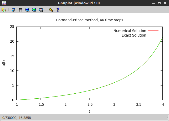
The exact solution to the ODE is \(y(x) = x\tan(\log(x))\). I plotted the obtained numerical solution and the exact solution using the Ruby gem gnuplot (Ruby code at the bottom of the page). One can clearly see that the Dormand-Prince solution agrees with the exact solution.

Using the exact solution, we can compute the error of the numerical solution. We can print further information about the obtained solution to the screen, using some of the attribute readers of Ode.

In particular, we see that the error of the numerical solution stays below the prescribed tolerance level, as intended.
Automatic step size adjustment
We look at a second example that demonstrates the automatic step size adjustment capabilities of the Dormand-Prince method. Suppose we have the initial value problem:
- ODE: \(\frac{dy}{dx} = -2y + e^{-2(x-6)^2}\), \(0 \leq x \leq 10\),
- IC: \(y(0) = 1\).
We apply the Dormand-Prince method with error tolerance 1e-6:
f = proc { |t,y| -2.0 * y + Math::exp(-2.0 * (t - 6.0)**2) }
dopri_sol = Ode.new(xrange: [0.0,10.0], dx: 1.5, yini: 1.0,
                    tol: 1e-6, maxiter: 1e6, &f)
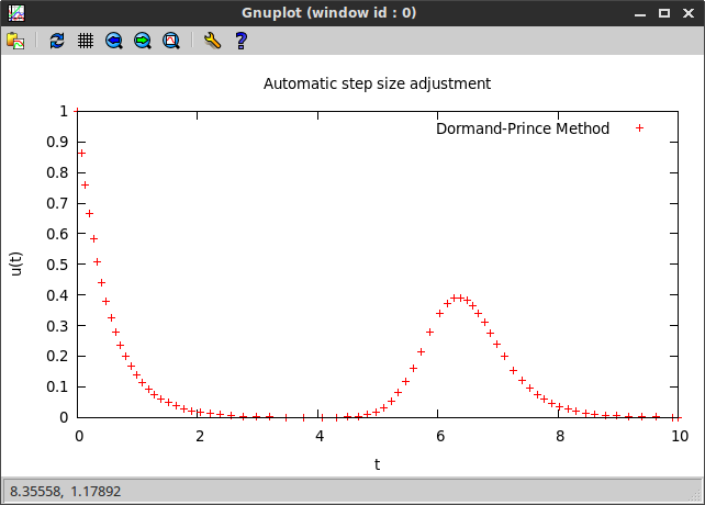
and plot the obtained solution on the grid generated by the method:

One can clearly see that the step size decreases in regions of bigger change in the slope of the function.
Euler method
The Euler method is the most basic method for solving ordinary differential equations. In its implementation in spitzy, unlike the Dormand-Prince method, it cannot automatically control the step size or estimate the error of the obtained numerical solution. We apply it to the same differential equation as in the Dormand-Prince example above.
f = proc { |t,y| 1.0 + y/t + (y/t)**2 }
euler_sol = Ode.new(xrange: [1.0,4.0], dx: 0.01,
                    yini: 0.0, method: :euler, &f)
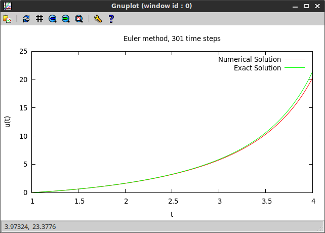
If we plot the obtained numerical solution, we can see that, even though the Euler method evaluates the solution at a much finer grid, it performs much worse than the Dormand-Prince method.

Nevertheless, there possibly are situations in which the simple Euler method is preferred over the rather complex Dormand-Prince.
Adams-Bashforth method
The Adams-Bashforth method implemented in spitzy is a second order method from the family of multi-step methods. As the Euler method, it operates on a fixed pre specified step size.
We demonstrate it by solving the following differential equation:
- ODE: \(\frac{dy}{dx} = -2xy\), \(0 \leq x \leq 4\),
- IC: \(y(0) = 1\).
The implemented Adams-Bashforth scheme is a method of order two, which means that the error of the numerical solution is proportional to the square of the step size. Consequently, if we halve the step size, then the error of the numerical solution should reduce by a factor of four. We check this theoretical property by computing two solutions with step sizes 0.1 and 0.05, and comparing their errors (the exact solution is \(y(x) = e^{-x^2}\). The following short code carries out the calculation, and its output is shown below.
require 'spitzy'

f = proc { |t,y| -2.0*t*y }
ab2_sol1 = Ode.new(xrange: [0.0,4.0], dx: 0.1,
                  yini: 1.0, method: :ab2, &f)
ab2_sol2 = Ode.new(xrange: [0.0,4.0], dx: 0.05,
                   yini: 1.0, method: :ab2, &f)

exact_sol1 = ab2_sol1.x.map { |tt| Math::exp(-(tt**2)) }
maxerror1 = exact_sol1.each_with_index.map {|n,i| n - ab2_sol1.u[i] }.max.abs
exact_sol2 = ab2_sol2.x.map { |tt| Math::exp(-(tt**2)) }
maxerror2 = exact_sol2.each_with_index.map {|n,i| n - ab2_sol2.u[i] }.max.abs

puts "Number of x steps: #{ab2_sol1.mx} and #{ab2_sol2.mx}"
puts "Error: #{maxerror1} and #{maxerror2}"
puts "Error ratio: #{maxerror1/maxerror2}"

As expected the error ratio is close to 4.
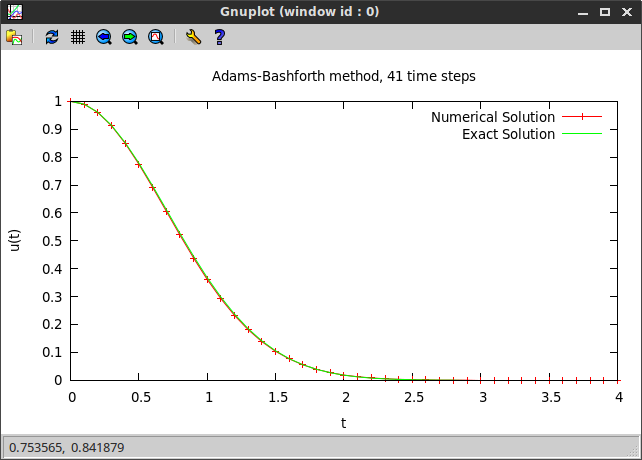
We also plot the numerical and the exact solutions.

All plots were done using the Ruby gem gnuplot and the following helper function.
# plot the numerical and the exact solutions
def plot_ode(x, numsol, exactsol, title, num_with="lines")
  Gnuplot.open do |gp|
    Gnuplot::Plot.new(gp) do |plot|
      plot.title title
      plot.xlabel "t"
      plot.ylabel "u(t)"

      t = x
      u = numsol
      plot.data << Gnuplot::DataSet.new([t,u]) do |ds|
        ds.with = num_with
        ds.title = "Numerical Solution"
      end

      y = exactsol
      plot.data << Gnuplot::DataSet.new([t,y]) do |ds|
        ds.with = "lines"
        ds.title = "Exact Solution"
      end

    end
  end
end